2 Data

2.1 Description

The data for this project comes from NYC Open Data, specifically the dataset titled “Jobs NYC Postings,” provided by the Department of Citywide Administrative Services (DCAS). This dataset is collected from information on current job postings available on the City of New York’s official jobs site (http://www.nyc.gov/html/careers/html/search/search.shtml), including both internal postings (restricted to city employees) and external postings (open to the public). The data is structured with categorical variables, such as agency/department and job title, and numerical variables, such as the number of positions and salary ranges. It consists of 5,560 rows and 30 columns and is updated weekly, with the most recent update on November 19, 2024. The dataset primarily includes job postings from 2024, which should not cause huge problems since outdated job postings would not be useful for this analysis. Potential issues include some missing or incomplete values that will need to be handled during the data cleaning process. To import the data, I downloaded the CSV file directly from the NYC Open Data portal (https://data.cityofnewyork.us/City-Government/Jobs-NYC-Postings/kpav-sd4t/about_data)

2.2 Missing value analysis

Code

library(ggplot2)

nyc_jobs <- read.csv("./Jobs_NYC_Postings.csv")

# turn all the empty cells into NA
nyc_jobs[nyc_jobs == ""] <- NA

missing_counts <- colSums(is.na(nyc_jobs))
missing_percentage <- (missing_counts / nrow(nyc_jobs)) * 100
missing_data <- data.frame(Column = names(missing_counts), 
                           Missing_Count = missing_counts, 
                           Missing_Percentage = missing_percentage)

missing_data_only <- subset(missing_data, Missing_Count > 0)

# plot 1: count of missing value for all columns
ggplot(missing_data, 
       aes(x = reorder(Column, -Missing_Count), y = Missing_Count)) +
  geom_bar(stat = "identity", fill = "skyblue") +
  coord_flip() +
  labs(title = "Count of Missing Values per Column", 
       x = "Columns", 
       y = "Count of Missing Values") +
  theme_minimal() +
  theme(
    axis.text.y = element_text(size = 8, hjust = 1)
    ) +
  scale_y_continuous(breaks = seq(0, max(missing_data$Missing_Count), by = 1000)) # Custom x-axis breaks

Code

# Second Plot: Pie Chart for Proportion
missing_data_only$Proportion <- missing_data_only$Missing_Count / sum(missing_data_only$Missing_Count)

ggplot(missing_data_only, aes(x = "", y = Proportion, fill = Column)) +
  geom_bar(stat = "identity", width = 1) +
  coord_polar("y", start = 0) +
  geom_text(aes(label = paste0(round(Proportion * 100, 1), "%")), 
            position = position_stack(vjust = 0.5), 
            color = "white", size = 4) +
  labs(title = "Proportion of Missing Values by Column") +
  theme_void() +
  theme(legend.title = element_blank())

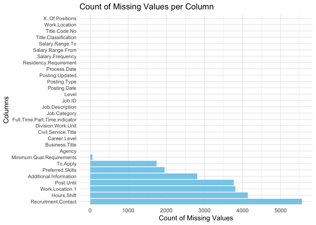
First graph: Count of Missing Values per Column

This bar chart shows the total number of missing values for each column in the dataset, knowing this is important because we’ll need to decide how to handle missing values, especially for columns with a lot of missing data. Specially, the column ‘Recruitment Contact’ has the highest count of missing values, with over 5,000 rows missing. This suggests the data for this column is almost completely unavailable. However, other essential columns like ‘Agency’, ‘Salary Range’, etc don’t have missing value, which is convient for later analysis.

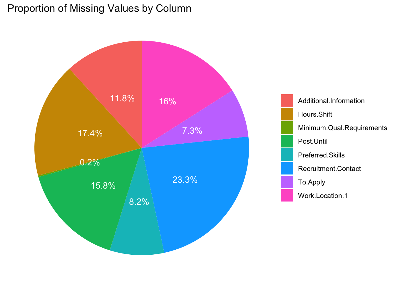
Second graph: Proportion of Missing Values by Missing Columns

This pie chart shows how much each column contributes to the total missing data, focusing only on columns with missing values. This chart helps us understand the overall impact of missing values from each column, so we can prioritize which ones to clean or exclude based on how much they contribute to the total missing data. Specifically, the “Recruitment Contact” column alone makes up about 23.3% of all missing data, which means it’s the most incomplete column in the dataset.